Summary
Integrates The IS-LM Model with the Phillips Curve into a unified framework. In the short run, IS-LM logic determines output; over time, the PC pulls the economy toward through inflation dynamics. Anchored expectations allow painless adjustment; de-anchored expectations require a recession. The zero lower bound can cause deflationary spirals, and oil shocks produce stagflation by shifting .
The name of the model explains what it is: an integration of The IS-LM Model with the Phillips Curve. We simplify by assuming the central bank sets the real interest rate directly (rather than the nominal rate , since ). The IS relation then becomes:
From Unemployment to the Output Gap
The IS-LM logic determines output in the short run, but supply constraints in the Phillips Curve prevail over time. Expressing things in terms of output rather than unemployment, we can write output and potential output as:
And the output gap as:
Which allows us to write the PC in terms of the output gap rather than unemployment:
Dynamics of the Model
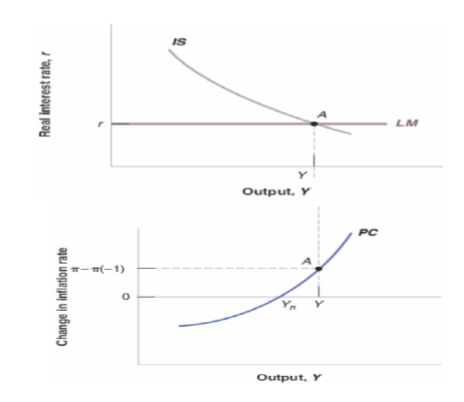
The IS-LM-PC model works in three steps:
- The central bank picks , which together with IS determines in the short run.
- The Phillips Curve then determines what happens to inflation: if , inflation rises; if , inflation falls.
- The central bank responds to inflation by adjusting , and the economy converges toward over time.
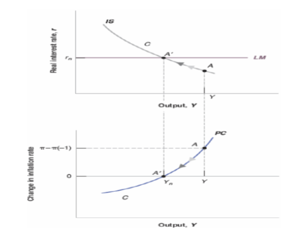
In the medium run, the economy settles at and . The real interest rate that achieves this is the natural rate of interest , defined as the rate consistent with in the IS relation.
If the central bank sets , output exceeds potential, inflation rises, and the bank must eventually tighten. If , output falls short, inflation drops, and the bank should ease. This is the core logic behind central bank policy rules like the Taylor rule.
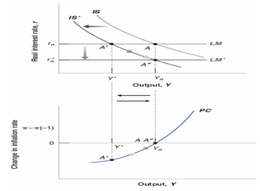
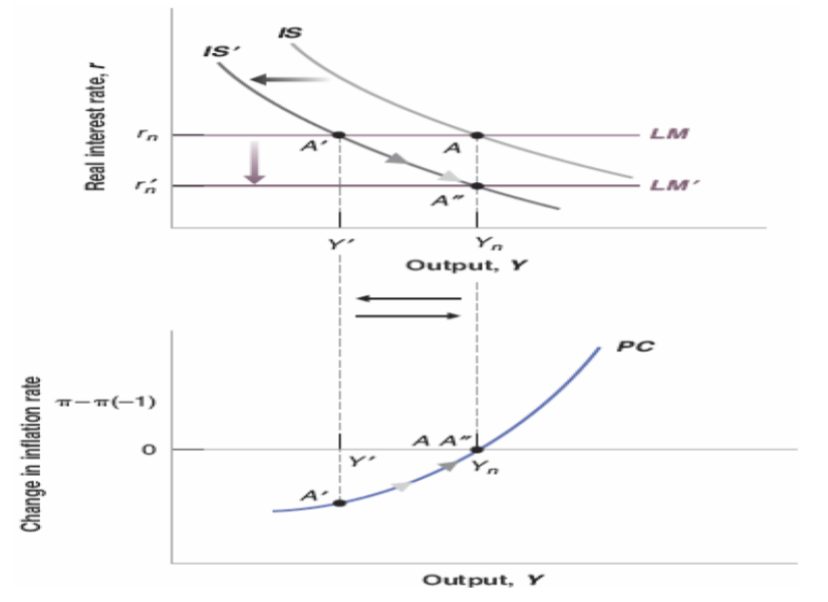
Example
Suppose (de-anchored expectations):
The lower graph explains why expansionary output won’t last forever. Inflation increases because of wage pressure. In order for output to return to equilibrium, the real interest rate must go up.
In the above example, we have an interest rate that is too low (). The natural rate (also called the Wicksellian interest rate) is defined implicitly from
where is the risk premium.
Anchored vs. De-Anchored Expectations
Whether adjustment is painless depends on how inflation expectations are formed.
 When inflation keeps rising despite rate hikes, the Fed is happy because , but unhappy because they might need to trigger a recession to bring inflation back down. This is why de-anchored expectations are dangerous. As long as inflation is anchored (, meaning people’s expectation of inflation doesn’t change), the economy can naturally return to without a recession.
In the medium run, real variables are independent of monetary policy (the Fed cannot permanently affect output). This is called the neutrality of money.
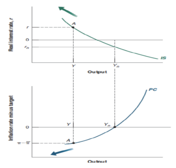
The Zero Lower Bound and Deflationary Spirals
Sometimes things go very wrong. If and inflation falls, the central bank wants to cut , but the zero lower bound on the nominal rate prevents this. Lower inflation raises the real rate (), which further depresses output, which further lowers inflation, creating a deflationary spiral.
 This happened most recently in Japan, and most notably during the Great Depression.
Fiscal Consolidation
Fiscal consolidation (raising or cutting ) is contractionary in the short run, shifting IS left. But in the medium run, the central bank can lower in response to falling inflation, bringing the economy back to at a lower real interest rate, further from the ZLB.
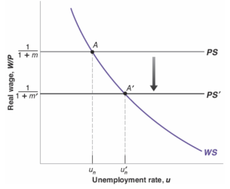
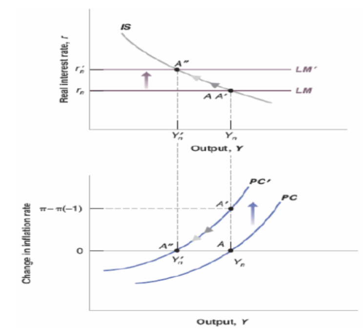
The Effects of an Increase in the Price of Oil
This leads to stagflation. The unemployment rate goes up because firms need to raise their markup to offset the increasing price of oil. This decreases the natural level of output, which shifts the Phillips Curve without shifting the IS curve, creating inflationary pressure at the same level of output.
A Persistent Financial Panic
A financial panic raises the risk premium , shifting the IS curve left. The central bank cuts to offset, but if the panic persists, may hit the zero lower bound.