Summary
Combines the goods market (IS) and financial markets (LM) to jointly determine output and interest rate in the short run. The IS curve is downward-sloping because higher reduces investment and output; LM is horizontal at the central bank’s chosen . Fiscal policy shifts IS, monetary policy shifts LM, and the two can be mixed to target different combinations of output and interest rate. At the zero lower bound, monetary policy loses traction (liquidity trap) and fiscal policy must step in.
Monetary policy is the chief tool for preventing cyclical economics. Sometimes, it’s not enough, in which case fiscal policy can also help. As a result, we need to look at the goods and financial markets together. This will help us understand the joint determination of output and interest rate in the short run, particularly with regard to the impact of monetary/fiscal policy on aggregate demand. Hicks and Hansen called this idea the IS-LM model.
The IS Relation
This is just the goods market, but rather than assuming investment constant, we replace it with a function:
This results in the equilibrium being modeled as
We now capture all combinations of and that are consistent with equilibrium in the goods market. As a result of the interest rate now being a parameter, the curve from Lecture 3 now is more dynamic:
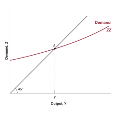 Not only is steeper but is no longer linear as interest rate changes, since high interest rate lowers demand. This is our IS relation.
Why is the IS curve downward sloping?
An increase in reduces investment, shifting down to and lowering output from to . Mapping these pairs into panel (b) traces out the downward-sloping IS curve.
What shifts the IS curve?
An increase in taxes reduces disposable income and consumption, lowering demand at every interest rate. The IS curve shifts left from to . A decrease in would produce a similar shift.
Anything that happens in the goods market involves IS.
The LM Relation
Remember that equilibrium in the financial markets requires
Dividing by yields the LM relation:
In equilibrium, real money supply equals real money demand, which depends on real income and interest rate , so LM really captures all the combinations of and that are consistent with equilibrium with financial markets.
Note
In reality, central banks set and choose they need to make consistent with equilibrium.
This leads to a horizontal LM curve in the real world. The only thing that can shift the LM is if the central bank changes its mind and moves the interest rate.
IS-LM Equilibrium
Point is where both markets clear simultaneously as it lies on both IS and LM. Points along LM but not IS have financial market equilibrium but excess supply/demand in goods; points along IS but not LM have goods market equilibrium but financial market disequilibrium.
Contractionary Fiscal Policy
An increase in (or decrease in ) shifts IS left to . The economy moves from to along the LM curve: output falls from to while stays fixed.
With just IS or LM, we cannot say what the difference in output will be after a curve shift, as we have two unknown variables. We need both in order to set .
Mechanism behind the IS shift
Higher reduces consumption, shifting demand from down to . Equilibrium output falls from to . This happens for any given level of , so the entire IS curve shifts left.
Expansionary Monetary Policy
The central bank lowers to , shifting LM down to . The economy moves from to along the IS curve: output rises from to .
How the central bank implements expansionary policy
To lower to , the central bank increases money supply from to . Along the money demand curve , equilibrium moves from to .
Why monetary policy moves along the IS curve
Lower increases investment, shifting demand from up to and raising output from to . Since itself changed (not or ), this is a movement along IS, not a shift of IS.
Policy Mix: All in!
Combine expansionary fiscal policy (IS shifts right to ) with expansionary monetary policy (LM shifts down to ). Both push output in the same direction, moving from to with a large increase in .
The Liquidity Trap
When is near zero, becomes flat — people are indifferent between money and bonds (see liquidity trap). Increasing to or just moves along the flat portion (points , ) without lowering . Monetary policy is ineffective, so fiscal policy must be used instead.
Policy Mix: Fiscal contraction + monetary expansion
Contractionary fiscal policy shifts IS left to (, output falls). The central bank offsets this by lowering , shifting LM down to (). Output returns to but at a lower interest rate, useful when you want to reduce the deficit without sacrificing output.