Summary
Review
From Saving, Capital Accumulation, and Output:
Population Growth
Dividing by :
Rewriting and using :
where the approximation drops the small cross term. So the change in capital per worker is:
Total Factor Productivity
Technological progress can take many forms, including larger quantities of output per capital/labor, better/new products, or a large variety within products. In this course we will mostly capture the state of technology (A) in terms of labor-equivalence (as if we had more labor):
Essentially, is the amount of effective labor.
Recall that constant returns to scale implies . If you set , we obtain
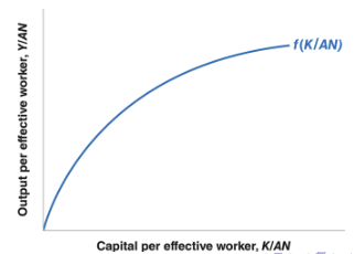
Capital per Effective Worker
Starting from and dividing by :
Using where :
where in the last step we set and to zero since these are small numbers. So the change in capital per effective worker is:
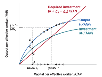
The steady-state growth of this economy can be found by setting the left-hand side to zero. Conceptually, this means investment is what is needed to cover the depreciation of the existing capital stock and catch up with the growth in effective labor (the denominator). Mathematically:
Steady-State Growth Rates
| Variable | Growth Rate |
|---|---|
| Capital per effective worker | |
| Output per effective worker | |
| Capital per worker | |
| Output per worker | |
| Labor | |
| Capital | |
| Output |
An Increase in the Saving Rate
What happens if increases from to ? The investment curve shifts up, so the new steady-state capital per effective worker is higher. Output per effective worker is also higher in the new steady state (compare with the no-growth case).
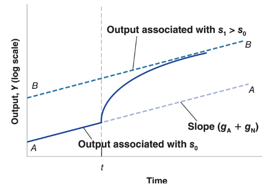 However, the long-run growth rate of output is unchanged: it remains . On a log scale, output jumps to a higher level but eventually returns to the same slope. A higher saving rate raises the level of output permanently but does not affect the growth rate in the long run.
An Increase in the Growth Rate of Effective Labor
What happens if increases? The required investment line pivots upward (steeper slope). At the old steady-state capital per effective worker , required investment now exceeds actual investment, so falls.
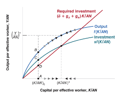 The economy converges to a new, lower steady-state with lower output per effective worker . Even though each effective worker has less capital, the economy grows faster in aggregate because is higher.
Balanced Growth
In the steady state, all variables grow at the rates given by the table above. We can verify this is internally consistent. For example, take . Then:
In balanced growth (steady state), , so:
which holds for any . This confirms that the growth rates in the table are consistent with the production function.
Measuring Technological Progress
Suppose each factor of production is paid its marginal product. It is then easy to compute the contribution of an increase in any factor of production to the increase in output.
Example
If a worker is paid
30k per year, her contribution to output is30k. If she works 10% more hours, her increase in output is $3k.
For labor, the contribution to output growth is:
Dividing by :
Letting (labor’s share of output):
Similarly for capital, since capital’s share is :
The Solow residual is whatever output growth remains after accounting for the contributions of labor and capital. It must be due to technological progress: