Neural Networks II

Summary

Backpropagation: computing gradients in neural networks via the chain rule. Builds on SGD by propagating error signals backward through layers, reusing intermediate results at each step. Dead ReLU neurons and vanishing/exploding gradients are key failure modes; skip connections help.

---

Recall that a fully-connected, feed-forward neural network has a layer of inputs, a linear combination of learnable weights and activation functions which form a layer, potentially many of such layers, and then an output.

Backward Pass

Backpropagation

The forward pass computes the output; the backward pass learns the parameters. We use SGD to update weights: randomly pick a data point , evaluate the gradient of its loss, and adjust toward optimality:

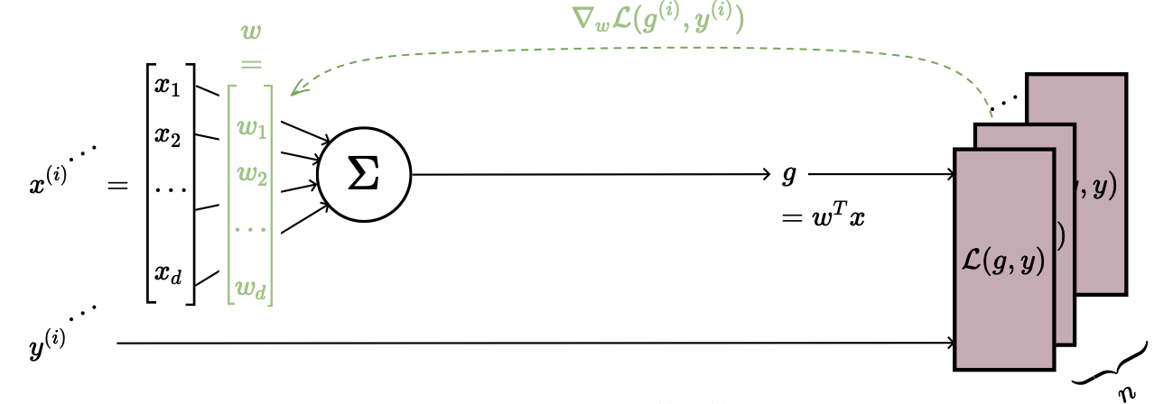
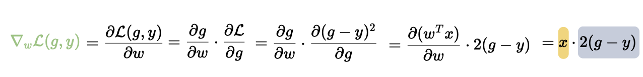
Suppose for simplicity that training data is just and squared loss. In this case, our gradient

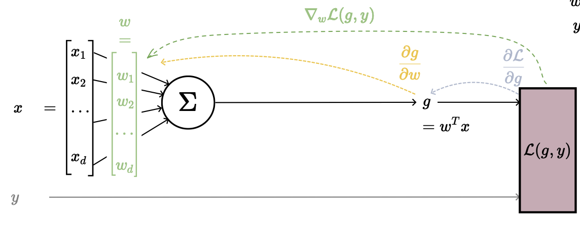
Slightly more interesting: We added a middle man here, which added another layer of complexity. This is the key insight behind backpropagation: the chain rule lets us decompose the gradient through each layer, computing partial derivatives one step at a time from output back to input.

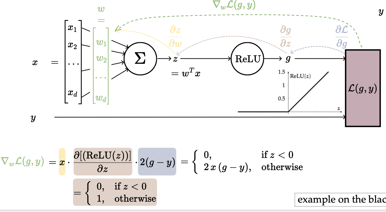
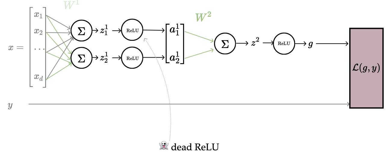
The problem here is that if the input to ReLU is negative, the derivative is zero, so there’s no update. This causes any downstream signal (from the term) to be nullified.

Recursive Reuse of Computation

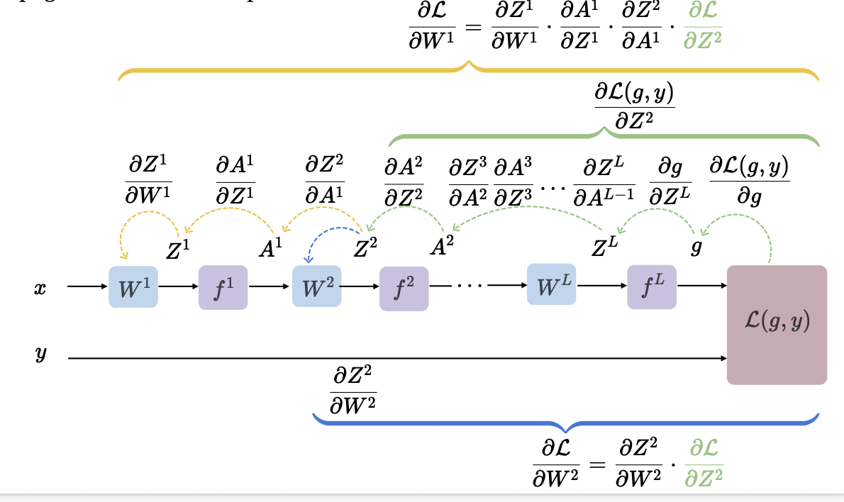
More abstractly, a backward pass runs SGD to update all parameters. We randomly pick a data point, evaluate the gradient , and update the weights. But how do we find ? 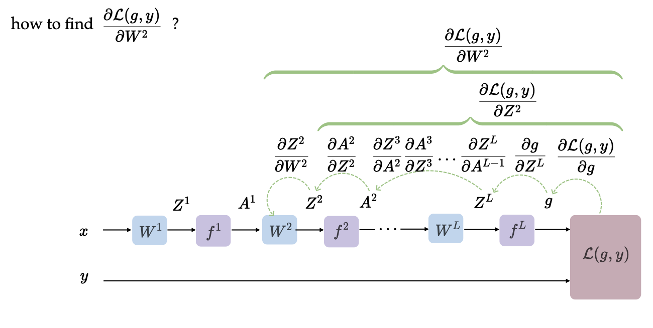We hop backward from the loss all the way to the beginning to recursively reconstruct the partial derivative. Now, how do we find ? We continue the same recursive loop. Since this is a chain reaction, we can reuse the layer-to-layer calculations we already computed.

To train a full neural network, we initialize our randomly. Then,

1. Forward pass: for each data point, compute
2. Evaluate loss: for each data point, compute .
3. Backward pass: pick a random data point, compute for all via the chain rule (reuse intermediate results, i.e. backpropagation)
4. Update: for all .

Gradient Issues and Remedies

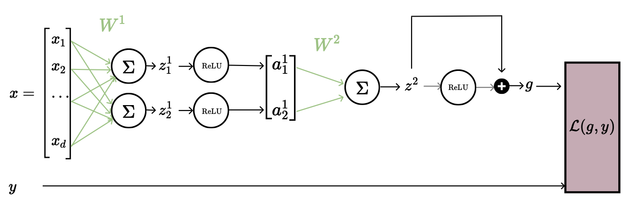
In the below example with more layers, if and , the grayed-out weights won’t get updated. If , no weights get updated at all. This follows from the same ReLU zero-derivative problem; we call this situation dead ReLU. The remedy: set , called a skip connection. Even with , the additive term lets gradients flow through, so earlier weights can still get updated.

There are also issues relating to vanishing or exploding gradients. Since the gradient is a product of per-layer factors (chain rule), if any factor is small the product shrinks quickly with depth, killing learning. Conversely, if factors are large, gradients explode. Both problems get worse as the network gets deeper. We can remedy this with residual connections or gradient clipping (if , rescale ).