Summary
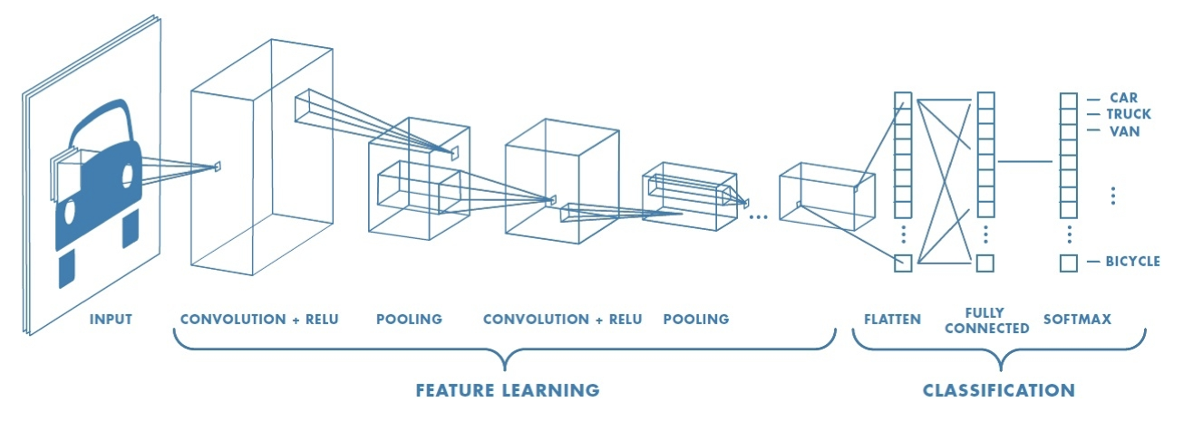
Even though neural networks are universal approximators, matching architecture to problem structure (visual hierarchy, spatial locality, translational invariance) improves generalization and efficiency. CNNs do this through convolution, which slides learned filters across the input to detect local patterns with shared weights, and max pooling, which summarizes spatial information (“did a pattern occur?” rather than “where exactly?”). Convolutional layers extract features; fully connected layers classify.
The course will become much less computational and significantly more conceptual. This week, we want to answer why we need a special network for images, and why CNNs are the special network for images.
Vision Problem
In order to pass even a small image into a fully-connected neural network, we need to do a ton of work. The number of parameters grows extremely fast. We need a specialized network because fully-connected nets don’t scale well and a carefully-selected hypothesis class helps fight overfitting.
Note
If we know the data is generated by a specific curve, we can more easily choose the appropriate hypothesis class.
So, do we know anything about our vision problems? Yes; there’s a natural visual hierarchy. 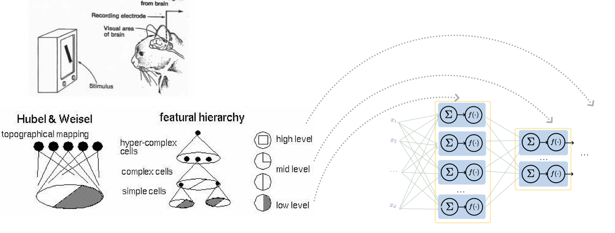 Turns out that the layered structure is well-suited for hierarchical processing. There’s also spatial locality in images. In other words, the distinguishing features can be found in neighborhoods rather than in arbitrary locations.
CNNs exploit visual hierarchy, spatial locality, and translational invariance through layered structure, convolution, and pooling to handle images efficiently. This punch line is a good template not just for images.
Typically, CNNs are a preprocessing block before a feedforward network we’re already familiar with to weed out the information that is relevant to us.
Convolution
1D & 2D Convolution
Convolution layers might sound foreign, but they’re actually very similar to fully-connected layers.
| Layer | Forward pass, do | Backward pass, learn | Design choices |
|---|---|---|---|
| fully-connected | dot-product, activation | neuron weights | neuron count, etc. |
| convolutional | convolution, activation | filter weights | conv specs, etc. |
| Convolution is akin to a filter applied to an image. |
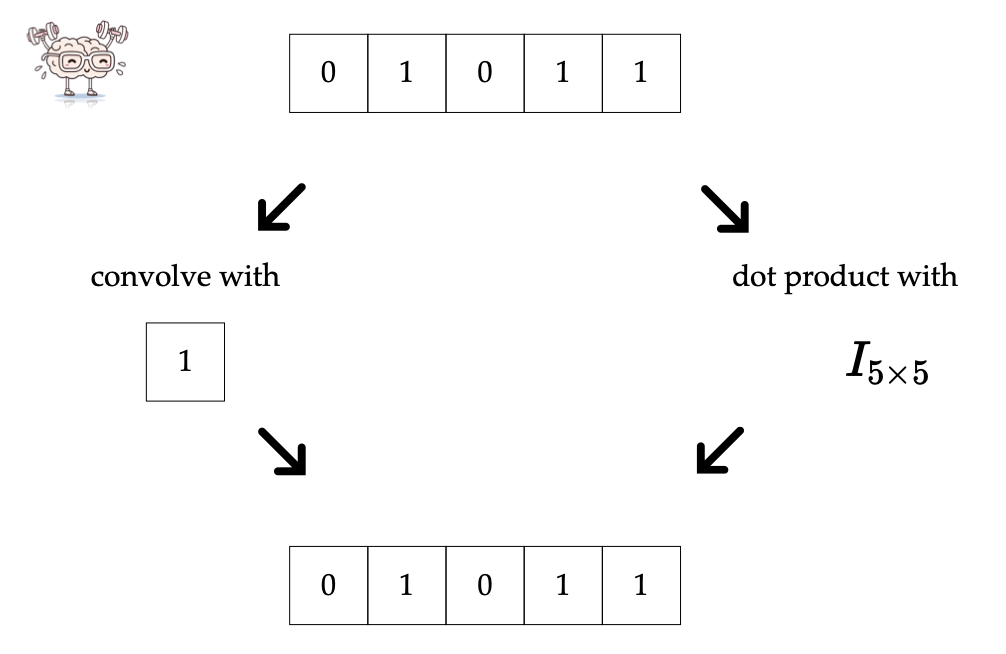
Example: 1D Convolution
Given input and filter , slide the filter across the input and compute the dot product at each position:
- Position 1:
- Position 2:
- Position 3:
- Position 4:
Convolved output:
There are four interpretations of convolution:
- Template matching
- “Looking” locally through the filter. This local region is called the receptive field.
- Sparse-connected layer with parameter sharing (dot product with mostly 0s)
- Translational equivariance
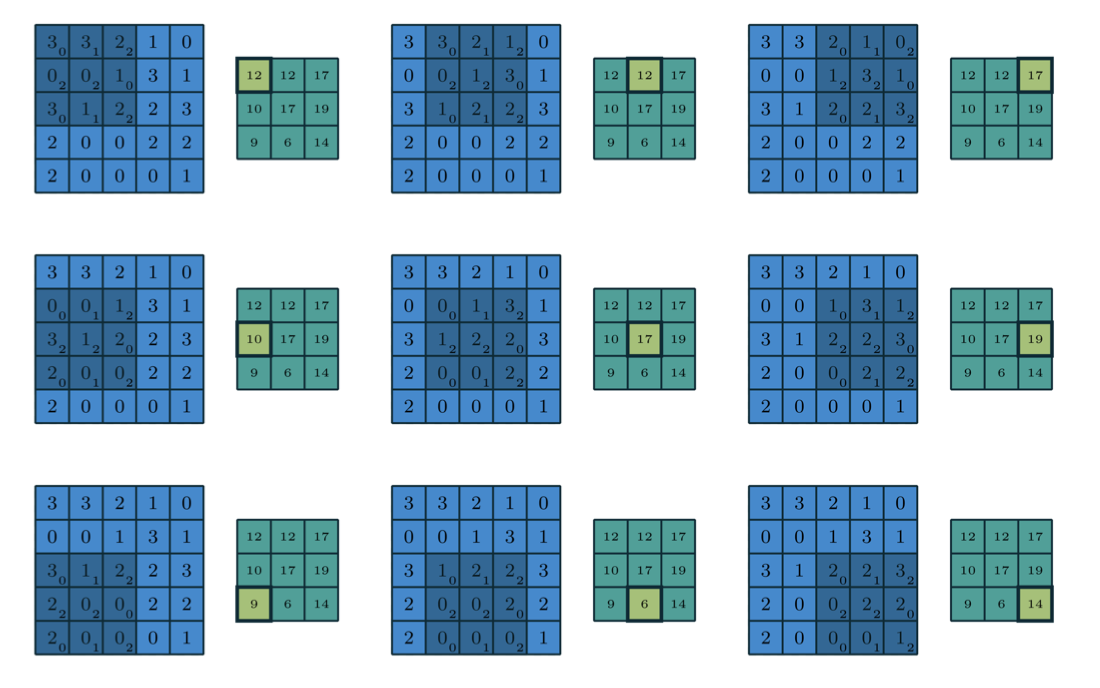
Example: 2D Convolution
Note
The stride need not be 1. It can be 2, 3, etc.
A summary of some 1D convolution techniques:
- Zero-padding: pad the input with zeros on both sides (e.g. ) so the output size is preserved
- Stride: how many positions the filter moves each step (e.g. stride of 2 skips every other position, reducing output size)
- Filter size: the number of weights in the filter (e.g. vs ). These weights are what the CNN learns during training.
In the old days, we hand-designed filters (Sobel). However, learned filters can find even non-obvious patterns.
3D Tensors
We don’t do 3D convolution. Tensors are a generalization of a scalar-vector matrix. 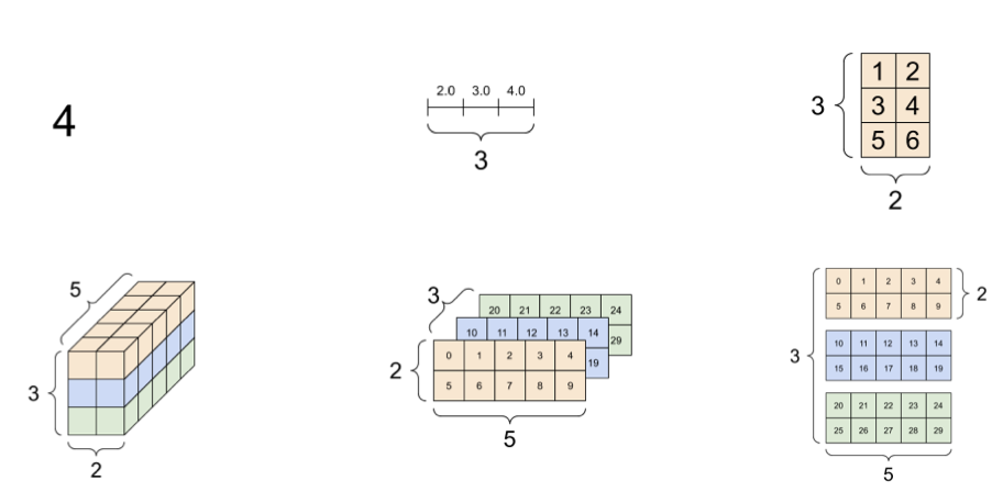 3D tensors hence are just a bunch of 2D matrices stacked. We will encounter these through color images (RGB). Each channel is a complete but independent representation of the scene. We can also get 3D tensors by using multiple filters, as different filters detect different patterns.
A fair question is why we don’t just do convolution in 3 dimensions. Remember that convolution shares weights across shifted positions. Hence, while which makes sense spatially (something can be anywhere), across channels it makes little sense (red is not green).
In full-depth 2D convolution, the input is a 3D tensor with channel depth , and the filter is also a 3D tensor with the same depth . We slide the filter spatially (height and width) but span the full depth, so the output of a single filter is a 2D matrix.
Applying multiple filters to the same input tensor produces multiple output matrices, one per filter. Each filter detects a different pattern, so we get one output channel per filter.
Stacking this together, an input tensor of depth convolved with filters (each of depth ) produces an output tensor of depth . The input depth matches the filter depth, and the number of filters determines the output depth.
Max Pooling
Convolution helps to detect patterns, but as we shift our pattern, the same filter keeps track of where it saw the object. Sometimes, we care about where something is, not just whether it exists. Pooling is just like convolution (sliding window) but there is no learnable parameter and it summarizes the strongest response.
Pooling across spatial locations achieves invariance with respect to small translations: 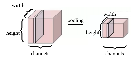 There’s a large response regardless of the exact position of the edge, so the channel dimension remains unchanged.