Summary
Linear programming is a technique to optimize linear objective functions subject to linear equality and linear inequality constraints. An instance of this is called a linear program (LP).
is the program with decision variables and a linear objective function with coefficients . There are linear constraints with coefficients , each using , , or . The last constraint is non-negativity: .
Example
You’re at your favorite arcade which houses two claw cranes and . If you spend on , you get stuff worth . If you spend on , you get stuff worth . You must spend at least as much on as you do on . You have at most to spend on and combined. Money spent on neither nor is lost. How do you get the most out of and ?
You want to put as much as you can in . However, since you need to put at least that much on , you put half into each.
Vectors and Matrices
For , of the same length , if and only if all components satisfy that relation.
Notation: is the zero vector, denotes a matrix, and is its transpose.
Maximization Standard Form
Minimization Standard Form
Let , , , . We can express the maximization standard form in 3 lines: , , .
Feasibility
A feasible solution is an satisfying and . The feasible region is the set of all feasible solutions. is feasible if , and infeasible otherwise.
Constraints can also be degenerate, meaning pulling them out doesn’t alter the feasible region.
Boundedness
is bounded if it fits in a finite ball, and unbounded otherwise. If is feasible, the largest value the objective function takes over the feasible region is the optimal value. A feasible solution achieving the optimal value is an optimal solution .
If is feasible and its optimal value is finite, is bounded, else it’s unbounded. If is bounded, it has an optimal solution and a unique optimal value. Multiple optimal solutions can give the same unique optimal value (degeneracy).
Geometric Visualization
n = 1
One decision variable .
Key takeaways:
- Feasible region is a convex set
- There is an optimal solution (if one exists) at a corner point As a corollary, there also can’t be two feasible regions.
n = 2
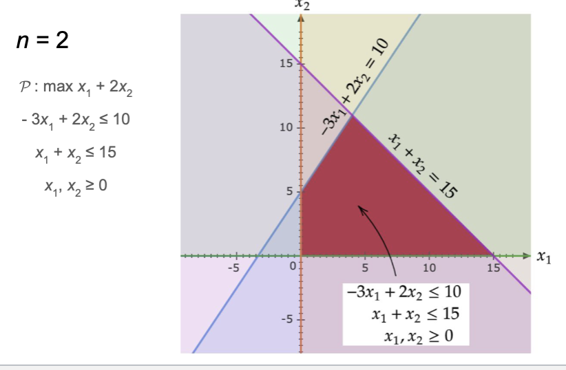 Notice that once again is a convex set and has an optimal solution at a corner point.
Solving Linear Programs
One of the first algorithms was the Simplex method which, though exponential time, is quite efficient in practice. It walks from corner to corner. The next is the Ellipsoid method, which, though polynomial, is often slow in practice. The class of methods used today is Interior-point methods, which are both polynomial time and efficient.
As a result, linear programs can be solved in polynomial time in the worst case.
Duality
Using the example, we have the optimal solution: 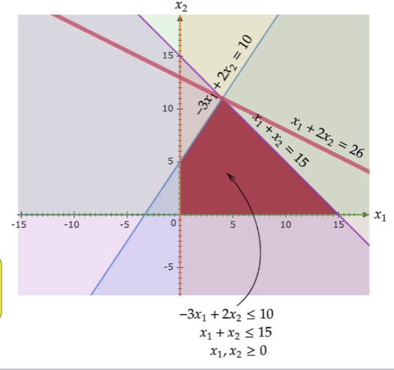 Note that since . This is close to the optimal value of 26. Let’s try again. .
One last time:
Note that since . This is close to the optimal value of 26. Let’s try again. .
One last time:
Hence, the optimal value is 26. Turns out we can always do this.
The general method gives us the dual program :
's optimal value 's optimal value
To see why:
since , , and . Rearranging:
since , , and . Therefore, the optimal value of .
Given a primal in maximization standard form:
the dual is the minimization problem:
There are primal constraints / primal decision variables ⇒ dual decision variables / dual constraints.
Note
The dual of the dual is the primal.
When a linear program is not in standard form, taking duals is a bit trickier. The general correspondence is:
| Primal (max) | Dual (min) |
|---|---|
| constraint | |
| constraint | |
| constraint | unrestricted |
| -th dual constraint | |
| unrestricted | -th dual constraint |
The dual objective is and the dual constraints come from vs , with the direction ( or ) determined by the table above.
Example
Note that is unrestricted (no non-negativity constraint). Applying the rules:
- Constraint 1 ()
- Constraint 2 ()
- Constraint 3 () unrestricted
- dual constraint 1 uses
- dual constraint 2 uses
- unrestricted dual constraint 3 uses
Duality Theorems
Weak Duality
If is feasible for and is feasible for , then .
Proof
The first inequality uses and . The second uses and .
What comes from this is that if is unbounded, then is infeasible. Additionally, if is unbounded, then is infeasible.
Strong Duality
If is bounded, then is also bounded and their optimal values are equal, denoted by and . Moreover,
This is the main mental model to keep: the primal is the thing you actually want, and the dual is a systematic way to prove you cannot do better. In max-flow terms, the dual object will turn out to be a cut.
Complementary Slackness
From the proof of weak duality, the two inequalities in the chain must both be tight at optimality (by strong duality). This forces:
Complementary Slackness
Let and be optimal for and respectively. Then for all and :
- — if the -th primal constraint is not tight, then
- — if the -th dual constraint is not tight, then
In other words, every dual variable “paired” with a slack primal constraint must be zero, and vice versa. This is useful for verifying optimality or solving for one solution given the other.
What are these s? Duality tells us which constraints to use to optimally bound the primal objective. It can tell us which primal constraints are degenerate (tossing them out keeps the optimal the same).
Minimum Spanning Tree Connection
Recall Minimum Spanning Trees. Today, we will assume all edge weights are positive and distinct. Kruskal’s algorithm repeatedly takes the minimum weight edge that doesn’t form a cycle until you get a minimum spanning tree. How can we connect this to linear programming?
Given , finding a minimum spanning tree can be seen as a decision regarding each , i.e. does or not, while maintaining the property that the edges chosen to be a part of and minimizing the total weight of the chosen edges.
Say we assign decision variables for all , that are basically indicators: if else 0. The problem is, how do we ensure the chosen edges form a spanning tree?
Let be a spanning subgraph of . A partition splits into disjoint parts, where for all . We say . Claim: if is a spanning subgraph, then for every partition , has at least edges crossing it. We also claim the reverse holds.
Claim: is a minimum spanning subgraph iff is a minimum spanning tree of . Check that for every partition , has exactly edges crossing it (a tree on vertices has edges, and each partition edge connects two parts).
This gives us the LP relaxation:
Note that we dropped the integrality constraint and relaxed it to . In general, LP relaxations give a lower bound on the integer optimum. The key result here is that this LP is integral: its optimal solution has for all , so the LP relaxation solves the MST problem exactly.
Theorem
The MST LP relaxation is integral, i.e. its optimal solution is the indicator vector of the minimum spanning tree.
To see why, consider the dual. There is one dual variable for each partition . The dual is:
By complementary slackness, at optimality:
- If (edge is in the tree), then (dual constraint is tight)
- If (partition is “active”), then (primal constraint is tight, i.e. the tree crosses with exactly edges)
This connects back to Kruskal’s algorithm: at each step, Kruskal picks the cheapest edge crossing some partition of the connected components. The dual variables can be interpreted as the “price” Kruskal’s algorithm pays at each merge step, and the algorithm implicitly constructs a dual feasible solution that matches the primal cost, certifying optimality via strong duality.