Summary
Derives short-run equilibrium output through the goods market. Aggregate demand, production, and income form a feedback loop. The multiplier amplifies changes in autonomous spending, and the paradox of saving shows that increased thrift can reduce output.
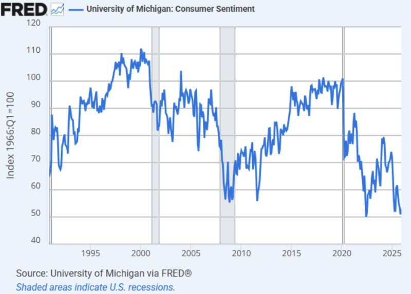
Consumer confidence is general sentiment of consumers in the United States. Despite not being in a recession, sentiment is quite low.
Before quiz 1, we will focus on the determination of equilibrium output across the short run, and later the medium and long run. In the short run, the main mechanism is the interaction between aggregate demand, production, and income. Changes in demand lead to changes in production. Changes in production lead to changes in income, and changes in income lead to changes in demand.

Composition of Aggregate Demand
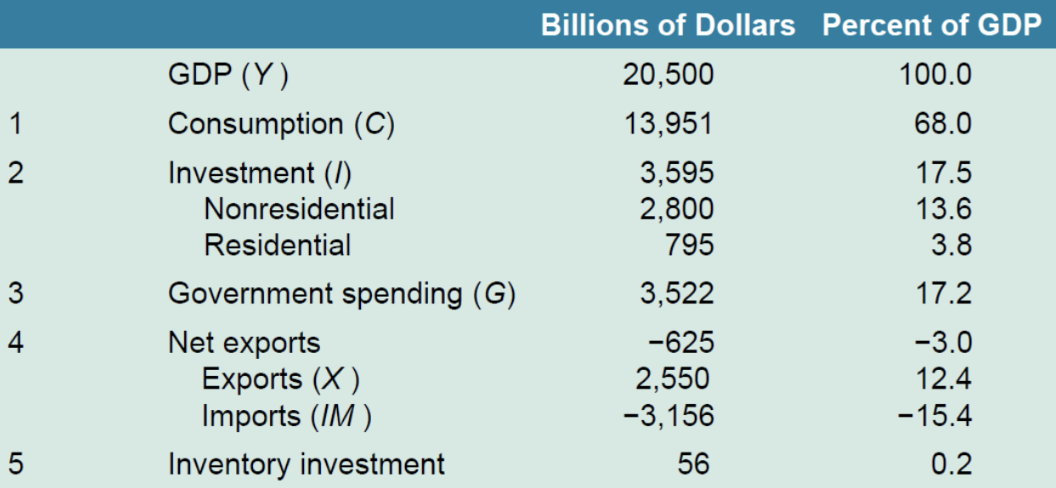
Building on our definition of GDP, aggregate demand is composed of:
- Consumption () — goods and services purchased by consumers
- Investment () — nonresidential and residential investment
- Government spending () — purchases by the government, excluding government transfers
- Exports () — purchases of US goods by foreigners
- Imports () — purchases of foreign goods by US consumers/firms/government
- Inventory investment — the difference between production and sales
Simplifying Assumptions
We set inventory investment to zero, and for now (closed economy).
US GDP Composition (2018)
In full:
In a closed economy:
Exogenous vs. Endogenous Variables
- Exogenous: determined outside the model, taken as given
- — investment is a fixed constant (the bar denotes it doesn’t respond to other variables; later we relax this in The Financial Markets)
- (government spending) and (taxes) describe fiscal policy
- Endogenous: determined within the model
- — consumption depends on disposable income
The Consumption Function
Assume consumption is linear:
- is autonomous consumption — independent of income
- is the marginal propensity to consume — how much additional consumption is generated by an extra unit of income
Disposable income is:
Substituting:
Note
can also be called output, since output is equivalent to income (see Basic Macroeconomic Concepts).
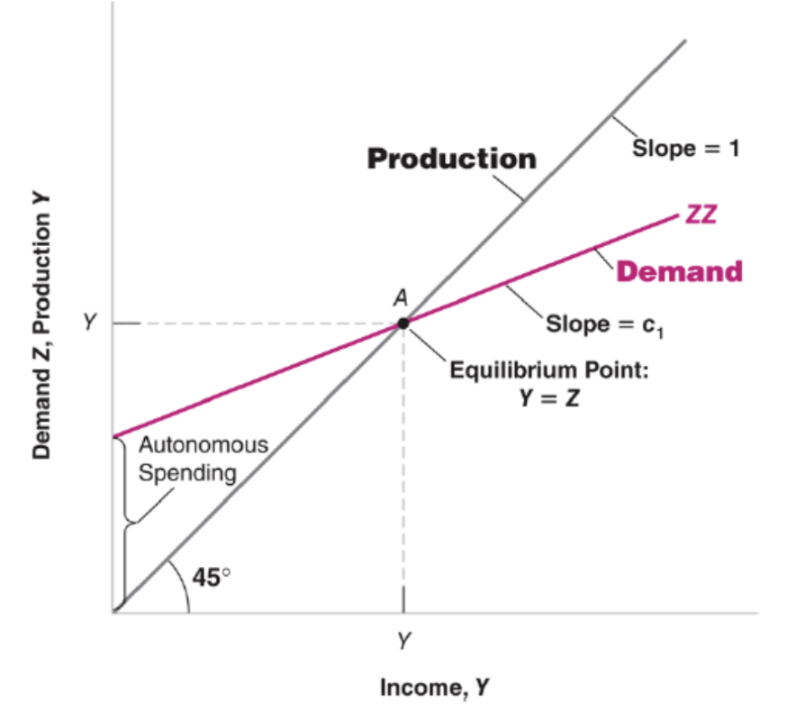
Equilibrium Output
Equilibrium in the goods market requires that demand equals supply: . This is not a function but an equilibrium condition. Output is demand-determined in the short run. Solving for output:
The term is the multiplier — a higher means a larger multiplier, amplifying any change in autonomous spending.
Note
This is the geometric series with ratio .
The relationship is recursive: more income means more demand, more demand means more output, and more output means more income.
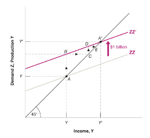
Shift in Autonomous Consumption
Suppose increases. The slope doesn’t change, but equilibrium demand shifts up.
$1 billion of extra income means $1 billion of extra output, leading to point C. But the effect doesn’t stop there — increased output raises income further, taking us from D to E, eventually converging to A’:
The IS Relation
There’s another way to determine equilibrium: find the output where investment equals saving. Private and public saving:
In equilibrium:
This is the IS relation, which implies — output equals aggregate demand.
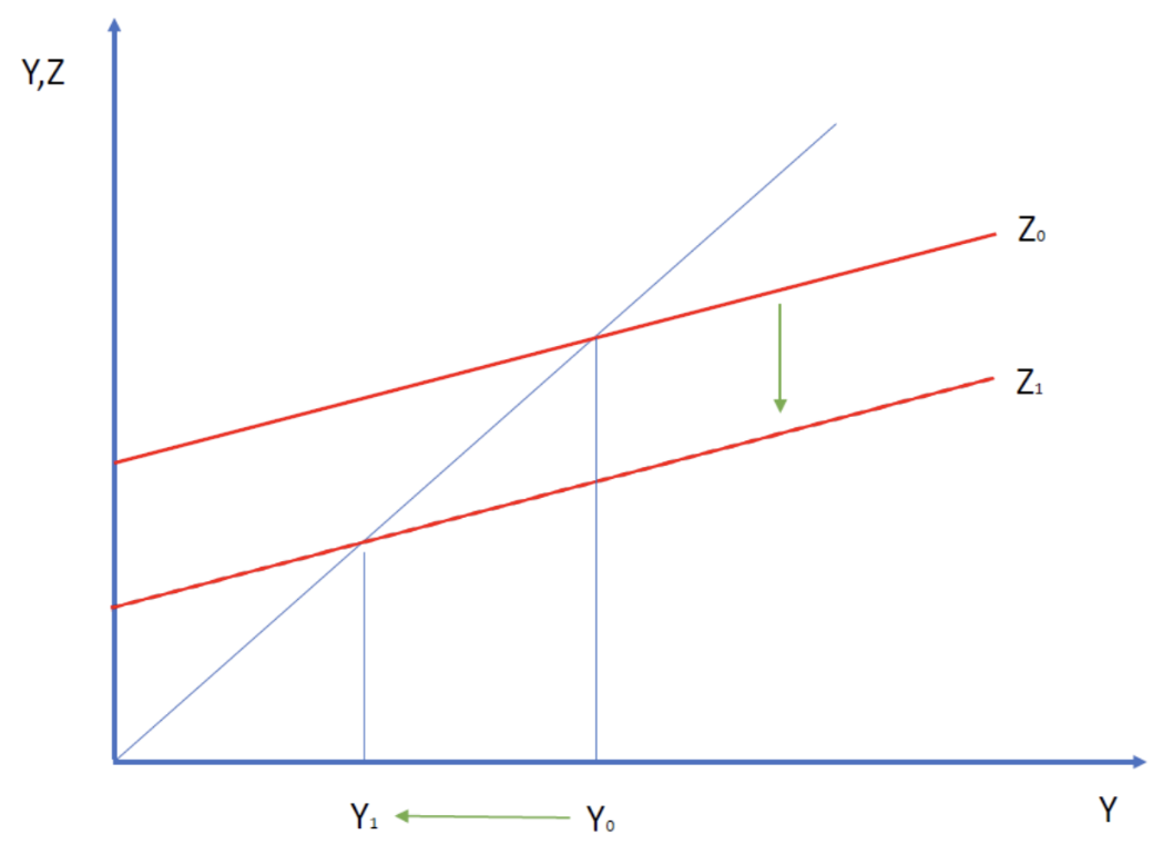
The Paradox of Saving
Since , saving is an increasing function of output — more income means more saving. However, in the short run:
As shifts up (people try to save more), must decline to restore equilibrium. Increased thrift reduces output — the paradox of saving.